How to use Pivot Tables in Excel 2007 and Excel 2010

Hi and welcome to my latest hub on Excel. Today I will examine the pivot table. Pivot tables are a very powerful way of presenting your data. They are far more versatile and flexible than a normal Excel table. It is this versatility that makes the pivot table so useful and also so powerful. With pivot tables:

• You can take a large amount of data and quickly and easily create focused reports based on any aspect of that data you choose
• The focus of your pivot tables can also be changed quickly and easily should you require different data to be displayed
• The table you create can be refreshed easily without the need to recreate or manually change it
• You can perform a number of statistical tests (SUM, COUNT, AVERAGE, MIN, MAX etc) on the data in your table
• Filters and sorting can also be used. Pivot tables make it easy to sort a column by the data held in another column

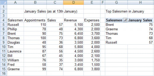
In today’s example, we will look at data from our team of salesmen. We will create a series of tables to illustrate how versatile and flexible pivot tables can be.

• First, we will look at sales for January
• Next, we will examine the top 5 salesmen for the same month
• Finally, we will show their expenses and also the average expenses for January

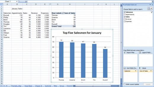
Pivot charts similarly are very versatile and work well with dynamic or frequently changing data. They allow you to display the results of a pivot table graphically (and therefore the underlying data source) and are as flexible and versatile as a pivot table. I have a hub that goes into Pivot charts into far more detail, including how to create, configure and refresh them. That hub can be found here:

http://robbiecwilson.hubpages.com/hub/Creating-Configuring-and-Using-Pivot-Charts-in-Excel-2007

To create a pivot table, first we need data we are going to use in our new table.

Note: Before creating a pivot table, ensure that each column has a title or Excel use the first row of your data as the column headers

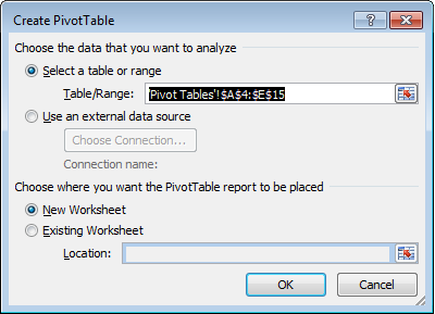
To create a pivot table:

• Select the data you intend to use to create it
• Choose Pivot table under the Pivot table button which is in the Tables Group on the Insert tab
• For Choose where you want the Pivot Table report to be placed, either, select a New Worksheet or a Location on an Existing Worksheet

Now we are presented with the Field list. We use this to build the table.

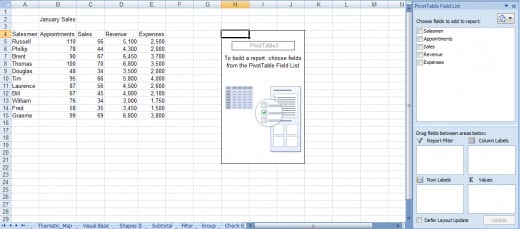
To begin with, we will create a simple table containing our salesmen and their sales.

• We select the check boxes for both and Excel builds a table for us

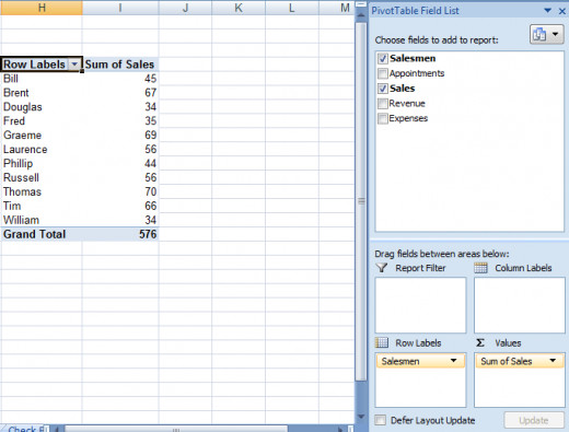
Note: If you click away from the table, Field list will close. To re-open it, click back on the table.

Now that we have created our table, we need to configure it to meet our needs. Firstly, let’s remove the Grand Total, as we don’t want to calculate that at this time. To do this:

• Right click anywhere on the pivot table and select Pivot Table Options
• On the Totals & Filters tab, clear the Show grand totals for columns
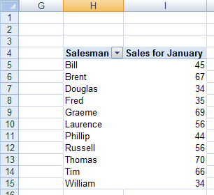
• We also want to rename the column header from Sum of Sales to Sales for January. Simply click on the cell and rename

Next, we will alphabetise the salesmen’s names. To do this:

• Select the names (cells H5 to H15) and click the Sort A to Z button on the Data tab in the Sort & Filter group

Now we have our pivot table completed.

Now suppose that we want to show the top 5 salesmen in terms of sales. Using the existing pivot table:

• Click the drop down box for the cell that contains the Salesman header (cell H4)
• Select Value filters
• Next, choose Top 10
• Change the Top 10 to be Top 5

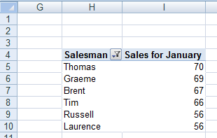
Now our table looks like this:

Note: the drop down box in H4 has changed its icon again to indicate that there are now two sorts on that column.

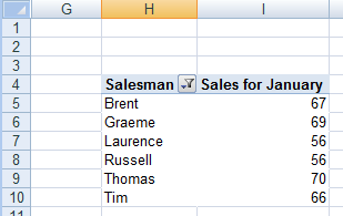
The table now shows the top 5, but they are not in order from highest to lowest as befits a top 5 list. To resolve this we will add a sort:

• Again, we click the drop down box in cell H4
• This time, we select More Sort Options

We want them in descending order and we want them sorted by their sales in January so:

• Select Descending (Z to A) by: and choose Sales for January

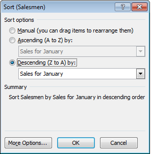
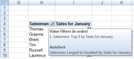
Note: To find out what filters or sorting has been applied, hover the mouse over the drop down box (e.g. H4) and Excel will display all those that have currently been applied.

Pivot tables become powerful when you have data that constantly changes or situations where you are called to produce multiple reports from the same data. We now have ours set up, but then our manager comes and asks us to produce a new report this time looking at the salesmen’s expenses for January. In addition, they want to know the overall average across all of the salesmen. To achieve this:

• First clear the filters on the Salesman column. To do this click on the drop down box and select Clear Filters from “Salesman”
• Next, clear the tick next to Sales in the Field list and select Expenses

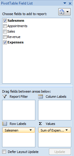
• Select the drop down box for Sum of Expenses in the Values box
• Choose Value Field Settings
• Click Average

Now we want to know the overall average, so we need to add the Grand Total back

• Right click anywhere on the pivot table and select Pivot Table Options
• On the Totals & Filters tab, select the Show grand totals for columns option
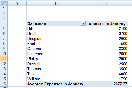
• Rename Grand Total (in cell H16) to Average Expenses in January

Alter cell I16 to show a number with two decimal places by:

• Right clicking and choosing Format Cells
• Select the Number tab and pick Number
• Rename cell I4 to Expenses in January

Now we have the following pivot table that we were able to configure quickly and easily:

Another key strength of pivot tables is how it deals with changing or dynamic data. Suppose due to an administrative error, Thomas’s expenses were 3,600 and not 3,500. If you used normal tables, you would have to update them manually. To update a pivot table:

• Select the pivot table
• Right click and choose Refresh

Excel will check the data source for the table and update any cells automatically

Should the need arise; you can easily change the data that Excel uses to create your pivot table to do this:

• Select a cell in your table
• Navigate to the Options tab which is part of the PivotTable Tools group of tabs. Click the Change Data Source button in the Data group

You can now adjust the cells you want to connect your table to.

If you are not happy with the position of your pivot table:

• Simply click on your pivot table
• Select the Options tab and the click the Move PivotTable button which is in the Actions group

If you decide that you are not happy with your pivot table and you want to start again and delete it:

• Select the entire table
• On the Home tab, in the Editing group, click the Clear All button and the pivot table will be deleted

Pivot table are immensely powerful and versatile. They offer several advantages over a standard Excel table:

• It is easy to create focused reports from large amounts of data
• Those reports can be quickly and easily changed to show different data as we showed above
• Pivot tables work brilliantly with dynamic or frequently changing data as they can be easily refreshed
• You can perform a number of statistical tests on the data in your pivot table including (SUM,COUNT, AVERAGE, MIN, MAX etc) which allows you to perform additional analysis
• Filters and sorting can be used to give users of your tables more useful information from the existing data

Thanks for reading my hub on creating and configuring pivot tables in Excel. I hope you have enjoyed reading my hub as much as I have enjoyed writing it and that you found it useful and informative. Please feel free to leave a comment below.